I. Preface
This article is a continuation of the article published at the beginning of this year, titledWhite-box part of DevSecOps constructionThis is a continuation of the previous article, in which the focus was on the construction of the automated process of code security detection, and only a brief mention was made of the implementation of the white-box engine technology, without a detailed explanation, without forming a complete knowledge system, so there is this continuation article.
At the beginning of the article, I want to talk about my demands on a code security analysis engine from the perspective of a user: the first point is that the rule writing should be simple and easy to use, and maintainable; the second point is that the CI/CD process embedding should be friendly; the third point is to support manual assisted audit; the fourth point is that the data analysis value should be great; the fifth point is that the analysis should be accurate; the sixth point is that it should be convenient for the team to quickly collaborate on development.

Starting from the first point, the requirement is that the rule writing should be simple and easy to use, and maintainable, so the addition of rules should be as parameterized as possible, and if it involves logical processing, it should be as simple as possible in the form of a script language.
The second point is that the process embedding needs to be friendly, so it requires that it be analyzed in a non-compiled manner, and the analysis speed needs to be as fast as possible.
The third point is to support manual assisted audit, that is, the engine is not only automated for audit, but also supports loading manual rule logic for secondary audit after the audit is completed, which can facilitate the colleagues in the red team to conduct vulnerability code audit and vulnerability mining;
The fourth point is that as an abstract code database, the potential value of data analysis is definitely great, so it is required that the data stored in the abstract code database be as comprehensive as possible;
The fifth point is that in order to ensure accuracy in analysis, the engine needs to establish a complete data flow diagram and be able to use the data flow path as an important basis for participating in the determination of vulnerabilities.
The sixth point is that it is convenient for the team to quickly collaborate on development, so the programming language used must be the most commonly used language in this field, and maintain a low degree of code coupling.
In response to the above demands of users, let's explore a tool that can not only meet the needs of enterprise internal automated audit, but also assist white hat hackers in quickly mining vulnerabilities. Then, I think, the best code security analysis engine for this is one written in Python, and the rules also support Python writing. The Aurora mentioned below is a code security analysis engine implemented by the author in Python. Of course, it is not all Python, the AST extraction is written in Java (which can be ignored), and the source code data analysis is written in Python.
Then, to get back to the point, how do we accurately analyze risk issues in the source code? I believe the most reliable basis is the complete data flow path. We know that sink points represent vulnerability points, and source points represent controllable entry points. If there is a data flow path from the source point to the sink, then we have reason to judge that there is a security risk at that location.
So how to obtain the complete data flow path? This requires a complete data flow graph and querying the path between the sink point and the source point according to the graph query algorithm. So how to build a complete data flow graph? This is a difficult problem and the main topic we will discuss today.
Before that, let's talk about the concept of code attribute graphs. I first learned about code attribute graphs from an open-source code security analysis project called joern by Fabian Yamaguchi. This project abstracts code and represents it in the form of a graph. Analysts can save the generated code attribute graph to graph databases such as janusgraph, neo4j, and orientdb, and use the gremlin graph query language for vulnerability analysis.
This is a very clever solution, but it also has some limitations in practice. Firstly, it needs to adapt to large-scale workloads, so the graph database must be provided in a cluster form. Cluster access involves network requests, and frequent requests for resources may trigger certain restriction strategies. If there is network latency, the speed of program analysis will be greatly slowed down.
Additionally, I feel that languages like gremlin have insufficient freedom in graph queries and are not very convenient to write rules. In recent years, a very good code security analysis software called codeql has emerged. Codeql itself provides a graph query language and offers very friendly rule writing plugins. From an overall perspective, the solution is somewhat similar to joern.
In practice, the effect of codeql is widely praised by industry professionals and has become a mainstream code vulnerability mining tool. However, if it is truly integrated into CI/CD, compilation issues may again become a hindrance to it.
The aurora code security analysis system implemented below may differ somewhat from the approach based on code attribute graphs. The main difference is that the data is not stored in a graph database, but in a large dictionary. The data structure of this dictionary is roughly as follows:
global_context={

  "job":{
      "job_id":"392302902332",
      "author_name":"pony",
      "project_name":"",
      "git_addr":"http://xxx",
      "branch_name":"xxx",
      "commit_id":"xxx",
      "start_time":"2021-12-31 00:00:00",
      "end_time":"2021-12-31 00:00:00",
    },
  "files":{
       file_id:{
         "file_name":"main.java",# Source code name
         "file_path":[path2file],# Source code path
         "source_file":""# If code collection is not allowed, it can be omitted.
               "job_id":""
       },
    },
  "classes":{
      "class_id":{
        "class_name":"",
        "package_name":"",
        "file_id":"32224423"
      }
    }
  "fields":{
      "field_id":{}# Omitted
    },
  "methods":{
      # Function summary information
      method_id:{
            "method_id": "",
            "method_name":"",# Function name
            "class_name":"", # Class name
            "package_name":"",# Package name
            "root_id": "",  # The default first node is the root node
            "ast_nodes": { # AST nodes,
                                      ast_node_id1:{},
                                                  ast_node_id2:{}
                                    },
            "is_dfa_analyzed": False, # Determines whether data flow analysis has been performed
            "CFG": {
                "block_nodes": {},  # Block node information,
                "block_contains": {},# Expressions included
                                                                "cfg_edges":{}, # Save control flow relationships
            },
            "dominant_tree": {},  # Dominant tree information, stored with direct dominance relationships
            "dominant_frontier": {},  # Dominant frontier information
            "call_graph": {},  # Control flow graph information
            "DFG": {
                'dfg_node': {},# Data flow graph nodes
                'def_use_edges': {},# Def-use edge relationships based on SSA form
                "pass_through_edges": []  # Data flow edge relationships added based on program data flow transfer rules
            }
        }
    },

   "components":{
      # Component Information Used in the Program, for Component Security Analysis
    },

   "results": {
        # Vulnerability Analysis Result
        "reports": {
             "xss":[
                                              {
                    "stainchain":"",# Stain Propagation Path
                    "sink":"",# Vulnerability Occurrence Point
                    "stain":"",# Stain
                    "flawsname":"",# Vulnerability Name
                    "description":"390390339",#vulnerability description information, place the description number, when displaying, index from the risk description dictionary by number.
                    'level':"5"#vulnerability level
                })
                                                 ]
        },
        "flaws_num": 0,
    }
}
In fact, this large dictionary is the code abstract database of aurora, based on which it is also very easy to generate a database in the form of code attribute graphs. During the actual analysis process, aurora will also generate some parts of code attribute graphs and perform data flow analysis and taint tracking based on code attribute graphs. In aurora's code attribute graph, callgraph, cfg, dfg, and dominantTree are all in independent graphs, so we can query the path between two nodes through simple graph query algorithms.
I will explain the structure diagram of this code data to lead everyone to understand the implementation principle of the Aurora static code analysis engine. The above code abstract database mainly contains the following parts:
components
methods
job
fields
classes
files
results
The 'components' section stores component dependency information, which is some component dependency information extracted from the configuration files of Maven or Gradle projects. The 'methods' section stores the most important abstract data, including function names, the scope of functions, various block nodes, expression nodes, and data flow nodes within functions, as well as the control flow edges between block nodes and the data flow edges between data flow nodes. In the data flow edge relationships, there are two parts of edge relationship sources, one part is from the data flow edge relationships generated by def-use analysis, and the other part is from the data flow path transfer rule analysis generated data flow edge relationships. The generation of def-use relationships depends on the SSA form of data flow analysis. To generate the SSA representation of the source code, it is necessary to generate the dominance tree based on the generated control flow graph, and then generate the dominance tree based on it, and then calculate the dominance boundary set based on the dominance tree, and then calculate the placement position of the phi function based on the dominance boundary set. Then, based on the dominance tree, construct the relevant algorithms for variable renaming. After renaming, you can traverse the control flow graph to generate the def-use chain relationship. The def-use chain generated based on SSA is simpler and easier to maintain than the def-use chain generated by the traditional data flow analysis scheme. The 'job' section stores some relevant information about the job, including the address, branch, and commit number information of the target project. The 'fields' section contains field information of all classes. The 'files' section contains all file information. The 'classes' section contains all class information. The 'results' section contains analysis result information.
Two: Control Flow Graph Construction
The second part is the construction of the control flow graph. The most important link in building the control flow is the division of basic blocks.
After getting the above basic understanding, let's talk in detail about how to develop a white-box engine. The first step is to build the control flow, and the most important link in building the control flow is the division of basic blocks. In javaparser, 15 kinds of Declaration structures, 23 kinds of statement structures, and 35 kinds of expression structures are defined, respectively:
Declaration statement
AnnotationDeclaration
AnnotationMemberDeclaration
BodyDeclaration
CallableDeclaration
ClassOrInterfaceDeclaration
ConstructorDeclaration
EnumConstantDeclaration
EnumDeclaration
FieldDeclaration
InitializerDeclaration
MethodDeclaration
Parameter
ReceiverParameter
TypeDeclaration
VariableDeclarator
expression
ArrayCreationExpr
DoubleLiteralExpr
SuperExpr
BinaryExpr
UnaryExpr
AnnotationExpr
EnclosedExpr
SingleMemberAnnotationExpr
FieldAccessExpr
ArrayInitializerExpr
ArrayAccessExpr
NullLiteralExpr
ConditionalExpr
InstanceOfExpr
TypeExpr
CastExpr
AssignExpr
ThisExpr
MethodReferenceExpr
ClassExpr
ObjectCreationExpr
BooleanLiteralExpr
CharLiteralExpr
MemberValuePair
MethodCallExpr
VariableDeclarationExpr
NameExpr
NormalAnnotationExpr
StringLiteralExpr
LongLiteralExpr
MarkerAnnotationExpr
LiteralStringValueExpr
LiteralExpr
LambdaExpr
IntegerLiteralExpr
Statement structure
WhileStmt
UnparsableStmt
TryStmt
ThrowStmt
SynchronizedStmt
SwitchStmt
SwitchEntryStmt
Statement
ReturnStmt
LocalClassDeclarationStmt
LabeledStmt
IfStmt
ForStmt
ForeachStmt
ExpressionStmt
ExplicitConstructorInvocationStmt
EmptyStmt
DoStmt
ContinueStmt
CatchClause
BreakStmt
BlockStmt
AssertStmt
With so many syntax structures, it is imaginable how much effort is required to construct a complete control flow structure. However, do not be too afraid. In fact, these many syntax structures can be mainly divided into three types, namely simple statements, compound statements, and transfer statements.
Simple statements include variable declarations, assignment operations, function calls, etc. These statements are expression statements, and the linear sequence of statements composed of these statements can be directly merged into a basic block. Compound statements include if statements, for statements, while statements, switch statements, etc., which are the focus of the control flow construction algorithm. Among them, if statements and switch statements contribute branches to the control flow. For the if statement, we give an example. For example:
int a=1;
if(x>1){
    a=a+1;
}
else if(x<1){
    a=a-1;
}
else{
    a=0;
}
System.out.println(a);
By analyzing the above code, we can easily divide the code into five basic blocks, namely:
int a=1;  -> B1
a=a+1;    -> B2
a=a-1;    -> B3
a=0;      -> B4
System.out.println(a); -> B5
The corresponding generated control flow graph is as shown below
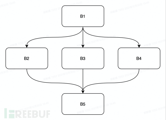
As shown in the figure, three branches extend from the basic block B1, corresponding to the three conditional branches in the if statement, and finally the three branches converge to the basic block node B5. Other statements can be divided into code blocks according to their own understanding.
Third, process data flow graph construction
It is not enough to have a control flow graph. To determine whether a vulnerability exists and reduce the false positive rate, taint tracking is indispensable. And to do taint tracking, it is necessary to establish a complete data flow graph. Let's discuss how to build the process data flow graph within the process. Here, through comprehensive consideration, we have adopted the static single assignment (SSA) scheme to analyze the data flow relationship of the program.
SSA form is a middle representation form of source code. By converting the source code into SSA form, it can be very convenient and fast to perform data flow analysis. Converting source code into SSA form mainly involves five steps: the first step is to build the complete control flow graph within the process, the second step is to generate the dominance tree within the process, the third step is to generate the dominance boundary, the fourth step is to place phi functions, and the fifth step is to rename variables.
First, let's talk about the concept of dominance tree. However, when the concept of dominance tree is first proposed, many people may be confused. First, I will give a brief introduction to the relevant knowledge points of dominance relationship.
First, what is a dominance relationship?
In a graph, there are two points u and w. If it is necessary to pass through u from the source vertex of the graph to reach w, then we say that u dominates w.
Take the following figure as an example:

Then according to the definition of the dominance relationship, the dominance relationship in the control flow graph is as follows:
1 dominates 2, 1 dominates 3, 1 dominates 4, 1 dominates 5
2 dominates 3, 2 dominates 4, 2 dominates 5
Second, what is a direct dominance relationship
If u dominates w, and the other dominators of w dominate u, then the node u is considered to be the direct dominator of node w, represented as idom (w).
Let's still take the control flow graph in the previous text as an example, then the direct dominance relationship in the control flow graph is:
1 directly dominates 2
2 directly dominates 3, 2 directly dominates 4, 2 directly dominates 5
After understanding the above two definitions, it is not difficult to conclude the definition of the dominance tree:
Given a directed graph, a starting point S, and an ending point T, we need to find the points that must be passed through in all paths from S to T (i.e., the intersection of the point sets on each path), which are called dominance points. In short, if a point (i.e., a dominance point) is deleted, there is no path that can allow S to reach T. The tree formed by the dominance points is called the dominance tree. The two adjacent points on the dominance tree are directly dominated by each other. Therefore, it is not difficult to conclude that the dominance tree within this process is as follows:
It is easy to draw the dominance tree according to the definition of the dominance tree. So how to generate it through an algorithm? You can refer to the following brute-force algorithm for generation:
def ssa_dfn_compute(rootid:str,successors:dict) -> list:
    '''
    @rootid       id of root node.
    @successors   the successors of the target.
    Calculate dfn
    Recursive implementation of depth-first search
    '''
    def dfs(nodeid, nodelist):
        nodelist.append(nodeid)
        nexts=successors.get(nodeid)
        if nexts:
            for next in nexts:
                if next not in nodelist:
                    dfs(next, nodelist)
    nodelist = []
    dfs(rootid, nodelist)
    return nodelist

def dominant_tree_build(rootid: str, successors: dict) -> dict:
    '''
    @rootid       the rootid of the cpg.
    @successors   cfg edges {"node1":[node2,node3,...]}

    @description: Dominator tree construction, used for variable rename in SSA and placement of phi functions.
    It can be generated by edges {(idom(w), w)}. idom refers to the direct dominator node of w.
    Brute-force construction of the dominator tree algorithm
    1. First perform a dfs traversal on the directed graph to obtain the dfn sequence.
    2. Then for each node p in the dfn sequence, start traversing from the node and stop at this node.
    3. Then traverse the dfn sequence again, and for each node c that has not been visited, mark its parent node as node p.
    '''
    # Calculate the dfn sequence
    dfn = ssa_dfn_compute(rootid=rootid, successors=successors) # Control flow graph depth-first search sequence

    def isVisited(nodeid: str,visited_node_list: list) -> bool:
        # Determine if the node has been visited
        if nodeid in visited_node_list:
            return True
        else:
            return False

    def dfs(nodeid: str, visited_node_list: list) -> bool:
        # @nodeid              the node waiting to be visited.
        # @visited_node_list   the node which has already been visited.
        # Depth-first search
        # Perform a depth-first search on the control flow graph starting from the root node until the input parent node is reached.
        if not isVisited(nodeid=nodeid, visited_node_list=visited_node_list):
            visited_node_list.append(nodeid)
            nexts=successors.get(nodeid)
            if nexts:
                for next in nexts:
                    if not isVisited(next, visited_node_list):
                        dfs(nodeid=next, visited_node_list=visited_node_list)

    dominant_tree={} # Simple dictionary of dominance tree (similar to adjacency list representation)
    # dominant_tree stores all the relationships between directly dominated and directly dominating nodes, dominant_tree[id]=dominant.
    for parent in dfn: # Traverse the dfn sequence
        visited_node_list = []
        visited_node_list.append(parent)
        dfs(rootid, visited_node_list)
        # Traverse the dfn sequence, pointing the dominating nodes of all unvisited nodes to parent. These dominating nodes will be overwritten when traversing the subsequent nodes.
        for child in dfn:
            if not isVisited(nodeid=child, visited_node_list=visited_node_list:
                dominant_tree[child] = parent
    return dominant_tree
The above figure shows the algorithm for generating the dominance tree in Python, which already has very detailed comments, so there is no need to elaborate here.
What is the use of the dominance tree? It mainly serves the third step of constructing the dominance frontier set and the fourth step of placing the phi function.
Here, the concepts of dominance frontier and phi function may be a bit confusing to everyone. Therefore, before proceeding with the subsequent explanation, I will give a brief introduction to the concepts of both. The academic definition of a dominance frontier is: If A is a predecessor of B that does not strictly dominate B, then B is called the dominance frontier of A. The set of all dominance frontiers of A is denoted as DF(A). DF stands for dominace frontier. (The definition of strict dominance is: if x dominates y and x is not equal to y, then it is said that x strictly dominates y.) The purpose of calculating the dominance frontier is to determine the placement position of the phi function.
Then, what is the use of the phi function? The phi function is generally placed at the aggregation point of the path, playing the role of aggregating all reached variable versions and selecting variable versions. This is a key step in handling data flow transmission relationships on the branch for static single assignment. In the subsequent code logic after the aggregation point, there is no need to worry about which branch the variable usage comes from, as a new variable version will be redefined in the phi function expression, and the subsequent def-use chain construction can directly find the target def's use set by searching for the same variable name. The following is the calculation algorithm for the dominator boundary set:
class SSADFCompute:
    '''
    Processing dominator boundary set solution
    '''
    @staticmethod
    def fetch_idom_from_dftree(dominant_tree:dict, nodeid:str) -> str:
        '''
        @dominant_tree edges{idom}.
        @nodeid         target block node.
        @description:   fetch idom rel from dominance tree.
        '''
        return dominant_tree.get(nodeid) if dominant_tree else None

    @staticmethod
    def ssa_df_compute(precursors: dict, dominant_tree: dict) -> dict:
        '''
        @precursors the precursors of the target node.
        @dominant_tree edges{idom}.
        The purpose of dominator boundary calculation
        - Locate the place where the phi node needs to be inserted
        Dominator boundary calculation steps
        - Find the connecting point block in the control flow (multiple predecessors)
        - Calculate the dominator boundary set for each connecting point block, and other block nodes will naturally be calculated together in the traversal process.
        - The dominator boundary set of each block is represented by df(ni)
        - An efficient way to solve the dominator boundary set is to first find the predecessor node b1 of a certain connecting node b2 (excluding its direct dominator nodes), and then from the dominator tree, from
        b1 traverses upwards to its directly dominating node. Then b2 is added to the node reached during traversal. In this way, after traversing all connection nodes, the dominance frontier set of all nodes is solved.
        Key points of dominance frontier calculation:
        - Traverse all predecessors of the node except the directly dominating node.
        df Algorithm reference to Keith D. Cooper's paper 'A Simple, Fast Dominance Algorithm>
        Pseudo-code of the algorithm:
        for all nodes, b
            if the number of predecessors of b>=2
                for all predecessors, p, of b
                    runner <- p
                    while runner!=doms[b]:
                     add b to runner's dominance frontier set
                     runner=doms[runner]
        Key points of the algorithm extraction:
        1. Traverse all nodes to find nodes with multiple predecessors.
        2. Traverse these nodes upwards until the directly dominating node of the node (excluding the directly dominating node).
        '''
        df_dict={}
        def recursion_up(idom: str, precursor: list, xnodeid: str):
            '''
            @xnodeid    Connection node with two predecessors
            @precursor  Set of predecessor nodes of the node
            @idom       Directly dominating node
            @description
             - Recursively upwards until the dominating node
             - Add the node to the dominance frontier set of the nodes reached during traversal
            '''

            for parent in precursor:
                if parent!=idom:
                    if not df_dict.get(parent)::
                        df_dict[parent]=[]
                    if xnodeid not in df_dict[parent]:
                        df_dict[parent].append(xnodeid) # Add the dominance frontier to the node reached during traversal
                    pre=precursors.get(parent)
                    recursion_up(idom=idom, precursor=pre, xnodeid=xnodeid)
                else:
                    break

        for nodeid, precursor in precursors.items():
            if precursor:
                if len(precursor)>1:
                    # Get the direct dominator node
                    idom=SSADFCompute.fetch_idom_from_dftree(dominant_tree=dominant_tree,nodeid=nodeid)
                    # Recursively traverse upwards until the direct dominator node
                    recursion_up(idom=idom,precursor=precursor,xnodeid=nodeid)
        return df_dict
There are very detailed comments in the code, so I will briefly explain the logic of the algorithm. First, obtain the set of cfg relationships existing in the form of predecessor nodes, traverse this precursors, and if a node has two or more predecessor nodes, it is considered that there is a path aggregation point at this node.
Then, perform a recursive upward traversal on the control flow graph to the direct dominator nodes of the current node, and then place the node in the dominator boundary of the nodes passed during the traversal.
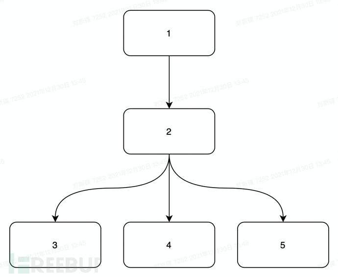
Taking the if statement code in the above text as an example, inserting a φ-function in its control flow graph results in the following figure:
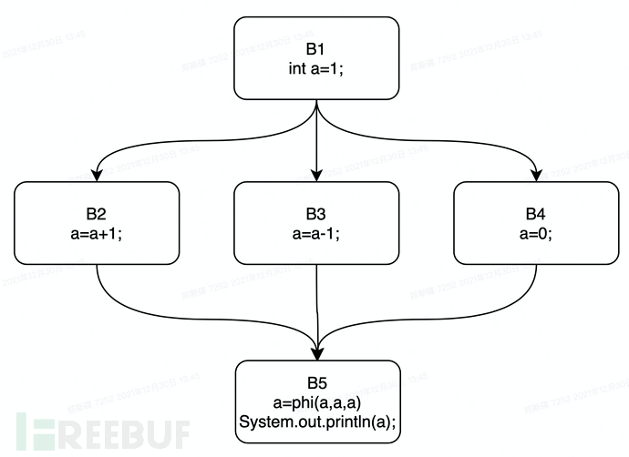
According to the definition of the dominator boundary, we can easily know that node B5 is the dominator boundary of B2, B3, and B4, so a φ-function should be inserted here to handle the static single assignment operations of multiple branches aggregated here. According to the definition of the dominator boundary and φ-function, we can easily mark the position where the φ-function should be placed in the graph. Then, how can we implement this process with an algorithm? You can refer to the following pseudocode for implementation:
function Place-phi-function(v) // v is a variable
    // For each variable in the control flow graph, execute this function to place φ-functions
    // has-phi(B, v)=true indicates that a φ-function has been placed in block B for the variable v.
    // processed(B)=true indicates that the variable v has been processed once on B.
    for all nodes B in the flow graph do
        has-phi(B, v) = false; processed(B) = false;
    end for
    W = ∅; // W is a work queue
    // Assignment-nodes(v) assignmnet-nodes(v) represents a set of nodes with assignment statements containing v.
    for all nodes B ∈ Assignment-nodes(v) do
        processed(B) = true; Add(W, B);
    end for
    while W != ∅ do
    begin
        B = Remove(W);
        for all nodes y ∈ DF(B) do
           if (not has-phi(y, v)) then // If the variable v has not placed the phi function on y
           begin
               place < v = φ(v, v, ..., v) > in y; # Place the phi function in the block y
               has-phi(y, v) = true;
               if (not processed(y)) then # If the basic block y has not been processed, then process y
               begin processed(y) = true;
                   Add(W, y);
               end
          end
        end for
    end
end
The following briefly explains the logic of the above code. For each variable in the control flow graph, execute Place-phi-function. In the logic of the Place-phi-function function, initialize the state for each node in the control flow graph.
It is necessary to set whether there is a phi function (set by the has-phi(B,v) function) and the function processed(B) is used to determine whether a node has been analyzed and processed. Then traverse all sets of assignment statements in the flow graph, push nodes containing copy statements onto the stack for processing, and then execute the phi function addition work for all dominating boundaries of the basic block B.
Here, since the renaming of variables has not been performed yet, it is currently unknown from which branch the parameters in the phi function come. So how to rename variables in expressions? You can refer to the following pseudocode to perform the rename operation:
function Rename-variables(x, B) // x是变量,B是基本块
begin
    ve = Top(V); // V 是x的版本栈
    for all statements s ∈ B do
        if s is a non-φ statement then // 如果s是未插入phi函数的语句(非赋值语句)
            replace all uses of x in the RHS(s) with Top(V);
            // Replace all uses of x on the right-hand side of the statement with the element at the top of the version stack.
        if s defines x then
        begin
            Replace the variable x with the newly defined version name xv, and push xv onto the version stack.
            v = v + 1; // v 是版本号计数器
        end
    end for
    for all successors s of B in the flow graph do // 对所有B在流程图中的后继节点执行
        j = predecessor index of B with respect to s
        for all φ-functions f in s which define x do
            replace the jth operand of f with Top(V);
            // Replace the parameters of the phi function with the variable version in Top(V)
        end for
    end for
    for all children c of B in the dominator tree do
        Rename-variables(x, c);
    end for
    repeat Pop(V); until (Top(V) == ve);
end
begin // calling program
    for all variables x in the flow graph do
        V = ∅; v = 1; push 0 onto V; // end-of-stack marker
        Rename-variables(x, Start);
    end for
end
A simple explanation of the logic of the aforementioned variable renaming algorithm. First, execute the Rename-variables function for all variables to perform the variable renaming operation. In the Rename-variables function, traverse all statements in the basic block B and perform the rename operation on the RHS of the statement. If the statement redefines the variable, then increment the variable index by 1 and push the variable onto the version stack.
Then, for the successor nodes of node B, if there is a phi function, rename the parameters in the phi function expression. If the phi function expression redefines the variable, then similarly, increment the variable version by 1 and push it onto the version stack. Then, perform the rename operation on all child nodes of basic block node B on the dominator tree through the Rename-variables(x, c) function. After that, execute the Pop(v) operation to restore the stack to the previous dominator node.
The aforementioned rename algorithm is not very complex, but it requires handling many details in practice. For example, when renaming the RHS in rename RHS, the statements provided are not all simple assignment statements. The RHS of the assignment statement may contain object creation statements and function call statements, and the function parameters are in Binary form. This requires us to consider multiple scenarios as much as possible, recursively parse and process the related statements, and rename the variables in the statements.
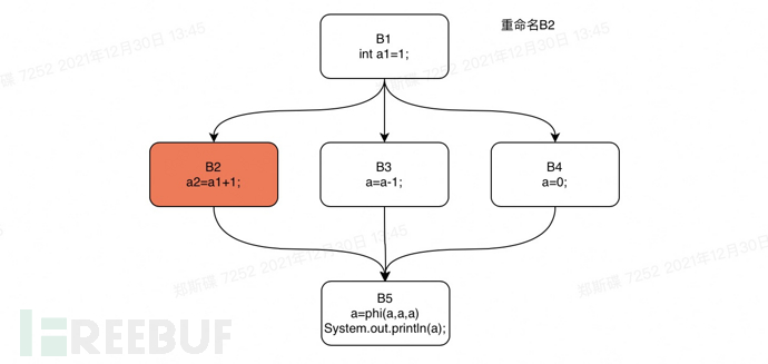
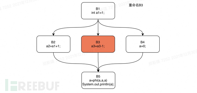
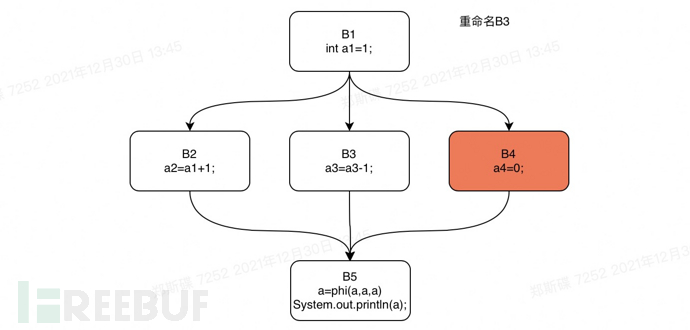
Next, we still take the if statement in the previous text as an example, and perform a rename operation on the control flow graph of this if statement. We will perform a depth-first traversal of the dominator tree of the if statement code starting from B1. The order of traversal is: B1, B2, B3, B4, B5.
Next, we can reproduce this process step by step.
Rename step1
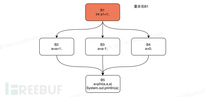
Rename step2
Rename step3
Rename step4
Rename step5
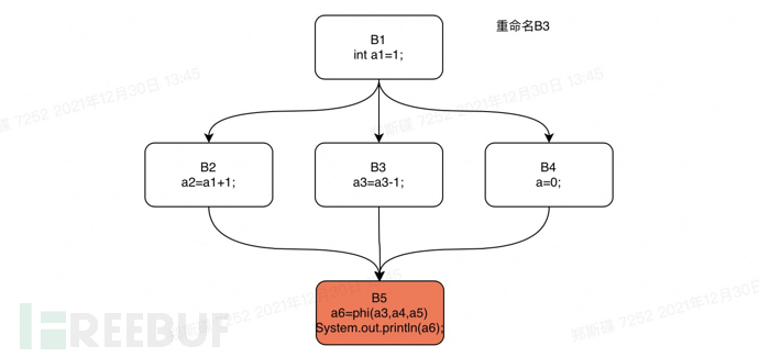
After the SSA form of the source code is constructed, we can then proceed to perform def-use chain analysis. The def-use chain generated by the SSA form analysis is particularly simple, because each variable's use has only one def, which means that as long as we traverse all the expression nodes in the control flow graph, collect the def and use information of variables, and then point the def of the same-named variable to the use.
Global Taint Analysis
The above text explains how to generate the def-use set of variables within the process based on the SSA form generation process. However, having only the def-use set is not enough to fully describe the flow relationship of data within the process. Because def-use only solves the problem that the variable use in the RHS is derived from which def above, but does not solve the problem that the def in the LHS comes from where, and whether there is a possibility of linking with the previous data flow path.
Firstly, for simple binaryExpr and nameExpr, we can easily connect RHS and LHS through assignment relationships, thus connecting the def in the LHS with the previous data flow. However, for some complex RHS, we can't easily connect RHS and LHS. For example, if the RHS is a methodcallexpr, and the variable exists in the parameters of the methodcallexpr, can we say that the parameters in the methodcallexpr will definitely have an impact on the LHS? Not necessarily.
So we need to provide it with some knowledge so that it can know that the parameter passed at a certain position of the function call will affect the LHS, thus establishing the relationship between the def in the LHS and the previous data flow path. According to my research, the majority of manufacturers basically complete this part of the data flow propagation relationship by supplementing the data flow flow rules. On the side of the R&D personnel of the engine development, they can generate this part of the data flow flow rules by parsing common java public class libraries. As for the library functions in other third-party SDKs, they need to be added by the subsequent maintenance personnel. Of course, someone may ask whether it can be automatically generated. Theoretically, it is possible, but in fact, the execution efficiency of the analysis engine will be greatly reduced.
After completing the data flow propagation within the process, we still cannot accurately find the vulnerability because in many cases, the source and sink points are not in the same function. This requires our engine to have the ability to perform inter-process analysis. Inter-process analysis is actually simple to say; we just need to establish the connection between the actual parameters at the function call location and the formal parameters at the function declaration location. In this way, the data flow graphs of the two processes are connected. However, it is noted that this connection needs to be established on the premise that the called function has also been parsed.
How do we ensure that the called function has been parsed? There are two solutions. One solution is to parse and mark the parsing status as true when encountering a function call, and the other solution is to directly parse all the processes required for the target vulnerability analysis. This requires establishing the necessary function call graph and then traversing the function call graph for process analysis. One of the benefits of generating a function call graph is that after we give a taint, we can generate all the processes that the taint may reach, which can give us a global grasp at the beginning. When we locate sink points later, we can traverse this call graph to find them, which will be much faster in terms of efficiency.
After establishing a global data flow graph, we can traverse the data flow graph for vulnerability analysis. So how do we perform the traversal analysis? How do we mark taints and sink points? Here, we need to define two data structures first. One is the data flow node, and the other is the AST node. The specific structure of the data flow node and AST node is not elaborated here, but it must contain an encoding parameter to identify the node, so that we can uniquely identify this node globally and avoid mistakenly traversing other nodes with the same name during data flow traversal. The information contained in the data flow node is relatively few. If we directly mark taints based on the name of the data flow node, the accuracy will be greatly reduced.
There is a solution to establish the association relationship between data flow nodes and AST nodes during the initial data flow analysis. Then, during the marking process, by analyzing the AST expression nodes, we can determine if the AST node contains a taint. If a taint exists, the corresponding data flow node can be marked as a taint. Of course, there is also another solution, which is to analyze whether a function call is a taint directly during the data flow analysis phase. If it is, a 'istaint' attribute can be marked on the data flow node. Similarly, if it is a sink point, it can also be marked with 'issink'. Subsequently, we only need to find out which nodes in the data flow graph are marked as 'istaint' and which are 'issink', and then analyze the data flow path between the taint and sink points through graph traversal algorithms.
Vulnerability rule engine section 5
A good rule engine can make the entire white-box engine more vibrant. For example, codeql, an open-source rule engine, uses DSL query language to write vulnerability rules and provides flexible API calls, which can greatly empower the knowledge of white-hat hackers to the engine, thereby enabling the engine to perform even better. However, although codeql is powerful, many people still think it is a waste of time to learn a DSL language that has no other application scenarios just to find vulnerabilities, so in the early stages of development, I decided that the plugin's script should be a very simple and easy-to-learn language, that is, python. I believe that the vast majority of people involved in network security-related fields will know python, right?
Below is the aurora rule engine (heavily inspired by the ideas of codeql, hahaha)
'''
XSS vulnerability detection rules
'''
from core.taintTrack.taintTracker import taintTracker
from core.dfa import dfa
from .base import base
class xss_rules(base):
    def __init__(self):
        self.name="xss"
        self.description="brief"
        self.advise="brief"
        self.level=5
        self.source_rule=[
            'getCookies', 'getRequestDispatcher', 'getRequestURI', 'getHeader', 'getHeaders',
            'getHeaderNames', 'getInputStream', 'getParameter', 'getParameterMap'
        self.sink_rule=["println"]
        self.clean=[]

        super().__init__(sink_rule=self.sink_rule,source_rule=self.source_rule,clean_rule=self.clean)
        # Data flow nodes
        self.sources=[]
        self.sinks=[]
        self.config_source_node()
        self.config_sink_node()
        self.config_clean_node()

    def check(self,graph:dict,method_id_list:list,rule:dict):
        '''
        Vulnerability detection
        '''
        taint_tracker=taintTracker(graph=graph,method_id_list=method_id_list,rule=rule)
        taint_tracker.taintTrack()  # Taint tracking
        taint_tracker.get_results()  # Results
        taint_tracker.env_clean()  # Clean the environment

    def config_source_node(self):
        # Start vulnerability analysis
        self.sources=self.search_source(
            global_context=dfa.DFGPathBuilder.global_context,
            source_rule=self.source_rule
        )

    def config_sink_node(self):
        '''
        Find sink points
        '''
        self.sinks=self.search_sink(
            global_context=dfa.DFGPathBuilder.global_context,
            sink_rule=self.sink_rule
        )

    def config_clean_node(self):
        dfa.DFGPathBuilder.global_context['clean_rules'] = self.clean
A brief introduction to the rule engine's approach: the three functions config_source_node, config_sink_node, and config_clean_node are used to configure taint points, sink points, and clean points respectively. The search_source function traverses the process expressions in the function call graph to find expressions with taints, and then marks the data flow nodes corresponding to the ast nodes during the subsequent data flow analysis construction. The same operation is performed for sink points and clean points. Users can add more taint marking logic by using the ast data access interface provided by the rule engine, and this part is also worth exploring in the future.
Of course, at the beginning, the plan was only to make the rules configurable, because it was thought that most of the supplementary capabilities, including rules, could be provided through configuration, such as Fortify, most of the rules are in the form of configuration. However, considering writing vulnerability detection plugins in script language, it may be able to integrate the knowledge and strength of white-hat hackers as well as codeql.
Personally, I think this white-box engine is quite promising later on. First, it doesn't need to be compiled, it directly parses javaparser to build data flow diagrams, and second, the rule script is written in Python, which is very friendly to white-hat hackers.
Six, About Open Source
This article is mainly to share the experience in white-box development over the past year, so that everyone who is still lost in the field can have a more systematic theoretical reference. As for open source, there is no plan for the time being. However, after a while, when the engine is more perfect and can contribute something to the community, it may consider open source.
Seven, References
https://groups.seas.harvard.edu/courses/cs252/2011sp/slides/Lec02-Dataflow.pdf
Eight, About Me
747289639@qq.com(WeChat same)
By Zheng Sidie
from Ideal Car Safety Department

评论已关闭