Author: Liu Huaining, JD Retail
Database Development History

Initially, data management was done through file systems, with data stored in files and both data management and maintenance carried out by programmers. Later, databases with tree-like and network-like structures were developed, but all of them had problems with expansion and maintenance. It was not until the 1970s that the theory of relational databases was proposed, organizing data in tabular form, with associative relationships between data, and possessing good structural and normalization characteristics, becoming the mainstream type of database.
Let's take a look at a timeline of database development first:
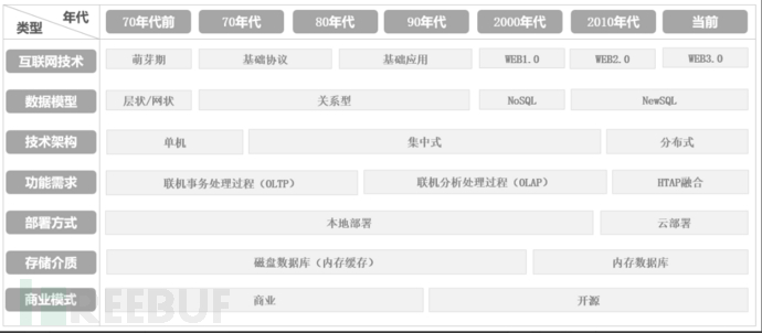
With the advent of the high-concurrency big data era, databases have been further refined and evolved according to various application scenarios. Typical representatives in the细分 field of databases include:
| Type | Product representatives | Applicable scenarios |
|---|---|---|
| Hierarchical Database (NDB) | IMS/IDMS | Data is organized in a tree-like structure, with parent-child relationships between data, resulting in fast query speeds but difficulty in expansion and maintenance |
| Relational Database (RDBMS) | Oracle/MySQL | Scenarios with transactional consistency requirements |
| Key-Value Database (KVDB) | Redis/Memcached | For high-performance concurrent read and write scenarios |
| Document Database (DDB) | MongoDB/CouchDB | For massive and complex data access scenarios |
| Graph Database (GDB) | Neo4j | Based on nodes and edges as storage units, efficient storage and query of graph data scenarios |
| Time-Series Database (TSDB) | InfluxDB/OpenTSDB | Scenarios for persistence of time-series data and multidimensional aggregation queries |
| Object Database (ODB) | Db4O | Supports complete object-oriented (OO) concepts and control mechanisms, with currently few usage scenarios |
| Search Engine (SE) | ElasticSearch/Solr | Suited for business scenarios mainly based on search |
| Column Database (WCDB) | HBase/ClickHouse | Scenarios for massive data storage and query in distributed storage |
| XML Database (NXD) | MarkLogic | Supports storage and query operations for XML format documents |
| Content Warehouse (CDB) | Jackrabbit | Large-scale high-performance content warehouse |
II Database Naming Concepts
RDBS
In June 1970, IBM researcher Edgar Frank Codd published the famous paper 'A Relational Model of Data for Large Shared Data Banks,' which marked the beginning of the software revolution of relational databases (Relational Database Server) software (previously dominated by hierarchical model and network model databases). To this day, relational databases are still one of the main data storage methods in the field of basic software applications.
Relational databases are based on the relational data model and are databases that utilize mathematical concepts and methods such as set algebra to process data. In relational databases, entities and their relationships are represented by a single structural type, which is a two-dimensional table. Relational databases store data in the form of rows and columns, with a series of rows and columns called tables, and a group of tables forming a database.
NoSQL (Not Only SQL) databases, also known as non-relational databases, emerged in the context of the big data era. They are capable of handling distributed, massive, uncertainly typed, and unguaranteed integrity
| Type | Product representatives | Application scenarios | Data model | Advantages and disadvantages |
|---|---|---|---|---|
| Key-value databases | Redis/Memcached | Content caching, such as sessions, configuration files, etc.; Frequent read and write, applications with simple data models; | Key-value pairs, implemented through hash tables | Advantages: Good scalability and flexibility, high performance; Disadvantages: Data is unstructured, can only be queried through keys |
| Column family databases | HBase/ClickHouse | Distributed data storage and management | Stored in column families, where the same column is stored together | Advantages: Simple, highly scalable, fast query speed; Disadvantages: Functional limitations, does not support strong consistency of transactions |
| Document databases | MongoDB/CouchDB | Web applications, storage of document-oriented or semi-structured data | Key-value pairs, where the value is a JSON structured document | Advantages: Flexible data structure; Disadvantages: Lack of unified query syntax |
| Graph databases | Neo4j/InfoGrid | Social networks, application monitoring, recommendation systems, etc., focus on building relationship graphs | Graph structure | Advantages: Support complex graph algorithms; Disadvantages: High complexity, limited support for data scale |
NewSQL
NewSQL is a category of new relational databases, which is a general term for various new scalable and high-performance databases. It not only has the storage and management capabilities of NoSQL databases for massive data, but also retains the ACID and SQL features supported by traditional databases, with typical representatives including TiDB and OceanBase.
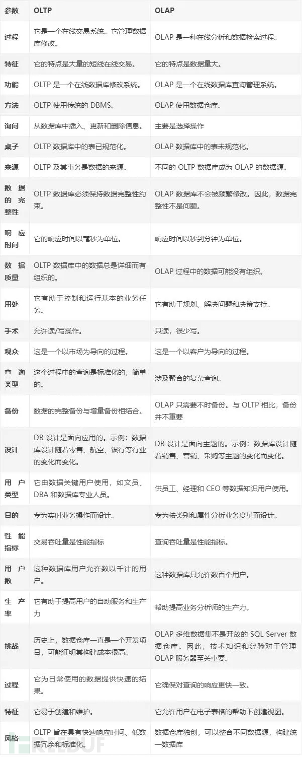
OLTP
On-Line Transaction Processing (OLTP): Also known as transaction-oriented processing, its basic feature is that the user data received on the front-end can be immediately transmitted to the computing center for processing, and the processing results can be given in a very short time, which is one of the ways to respond quickly to user operations.
OLAP
On-Line Analytical Processing (OLAP) is a process for data analysis that is oriented towards enabling analysts to observe information from all aspects quickly, consistently, and interactively, with the aim of gaining a deep understanding of the data. It has the characteristic of FASMI (Fast Analysis of Shared Multidimensional Information), which means fast analysis of shared multidimensional information.
Regarding the difference between OLTP and OLAP, the following table is used for comparison:
HTAP
HTAP (Hybrid Transactional/Analytical Processing) hybrid databases are based on a new computing and storage framework that can support both OLTP and OLAP scenarios, avoiding resource waste and conflicts caused by a large amount of data interaction in traditional architectures.
Three Domain Databases
Columnar databases
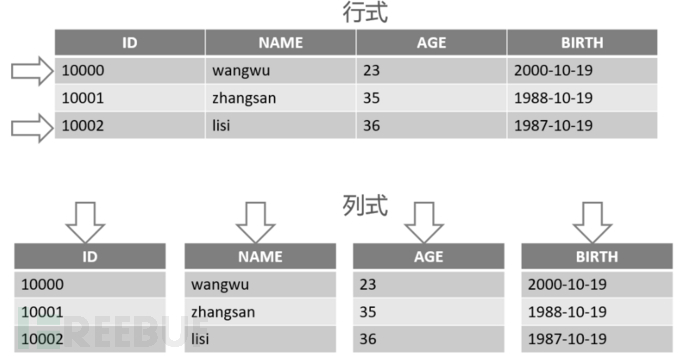
Traditional row-oriented data storage mainly meets OLTP applications, while column-oriented data storage mainly meets query-intensive OLAP applications. In columnar databases, data is stored by column, and the data type in each column is the same. This storage method enables columnar databases to process large amounts of data more efficiently, especially when large-scale data analysis and processing are required (such as in the financial, medical, telecommunications, energy, logistics, and other industries).
The difference between the two storage structures is shown in the following figure:
Main advantages of columnar databases:
・Higher compression ratio: Since each column contains data of the same type, columnar databases can use more efficient compression algorithms to compress data (compression ratio can reach 5~20 times), thereby reducing the use of storage space.
・Faster query speed: Columnar databases can only read the required columns, without needing to read the entire row of data, thereby speeding up query speed.
・Better scalability: Columnar databases can be easily horizontally scaled, that is, more nodes and servers can be added to handle larger-scale data.
・Better support for data analysis: Since columnar databases can handle large-scale data, they can support more complex data analysis and processing operations, such as data mining, machine learning, etc.
Main disadvantages of columnar databases:
・Slower write speed: Since data is stored by column, each write operation needs to write the entire column, not a single row, so the write speed may be slower.
・More complex data models: Since data is stored by column, the data model may be more complex than that of row-oriented databases, requiring more design and development work.
Application scenarios of columnar databases:
・Finance: Financial industry transaction data and market data, such as stock prices, foreign exchange rates, interest rates, etc. Columnar databases can process these data more quickly and support more complex data analysis and processing operations, such as risk management, investment analysis, etc.
・Medical: Medical industry病历data, medical images and experimental data, etc. Columnar databases can store and process these data more efficiently and support more complex medical research and analysis operations.
・Telecommunications: User data and communication data in the telecommunications industry, such as call records, SMS records, and network traffic. Columnar databases can process these data more quickly and support more complex user behavior analysis and network optimization operations.
・Energy: Sensor data, monitoring data, and production data in the energy industry. Columnar databases can store and process these data more efficiently and support more complex energy management and control operations.
・Logistics: Transport data, inventory data, and order data in the logistics industry. Columnar databases can process these data more quickly and support more complex logistics management and optimization operations.
In summary, columnar databases are a high-efficiency database management system for processing large-scale data, but it is necessary to weigh factors such as write speed, data model complexity, and cost. With the continuous development of traditional relational databases and emerging distributed databases, columnar storage and row storage will continue to merge, and database systems will present a dual-mode data storage method.
Time-Series Database
The full name of time-series databases is Time Series Database (TSDB), which is a specialized database for storing and managing time-series data. It is an optimized database for ingesting, processing, and storing timestamped data. Compared to conventional relational databases SQL, the biggest difference is that time-series databases are databases that record data at regular intervals indexed by time.
Time-series databases are widely used in scenarios such as IoT and internet application performance monitoring (APM). Taking data collection for monitoring as an example, if the data collection interval for monitoring data is 1s, a monitoring item will produce 86,400 data points per day. If there are 10,000 monitoring items, then a day will produce 864,000,000 data points. In the IoT scenario, this number will be even larger, with the scale of the entire data reaching TB or even PB levels.
History of Time-Series Database Development:
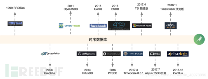
In the most common Kubernetes container management systems, it is usually paired with Prometheus for monitoring. Prometheus is a combination of an open-source monitoring & alerting & time-series database.
Graph Database
Graph databases (Graph Database) are a new type of NoSQL database based on graph theory. Both their data storage structure and data query methods are based on graph theory. In graph theory, the basic elements of a graph are nodes and edges, which correspond to nodes and relationships in graph databases.
Graph databases can perform very complex relationship queries in scenarios such as anti-fraud multi-dimensional association analysis, social network graphs, and corporate relationship graphs. This is because the graph data structure represents the inherent connections of entities, reflecting the essence of things in the real world. These connections are established at the time of node creation, allowing for quick paths to return associated data during queries, thus demonstrating very efficient query performance.
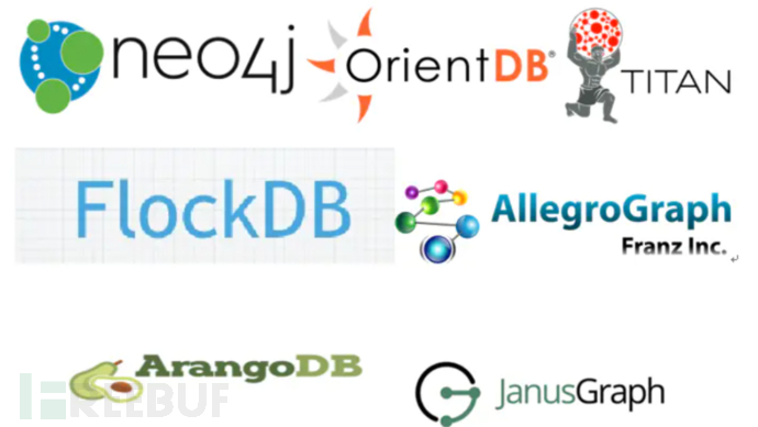
目前市面上较为流行的图数据库产品有以下几种:
与传统的关系数据库相比,图数据库具有以下优点:
1. 更快的查询速度:图数据库可以快速遍历图数据,找到节点之间的关联和路径,因此查询速度更快。
2. 更好的扩展性:图数据库可以轻松地扩展到大规模的数据集,因为它们可以分布式存储和处理数据。
Currently, some popular graph database products on the market include the following:
Compared with traditional relational databases, graph databases have the following advantages:
1. Faster query speed: Graph databases can quickly traverse graph data to find relationships and paths between nodes, so the query speed is faster.
2. Better scalability: Graph databases can easily scale to large datasets because they can store and process data in a distributed manner.
3. Better data visualization: Graph databases can visualize data as graphics, making it easier for users to understand and analyze data.
4. Better data consistency: Graph databases can ensure data consistency because they can establish mandatory relationships between nodes and edges.
Four Data structure design
| The previous section briefly introduced the basic knowledge of databases, and now we will introduce several common application practices related to data structure design: lookup tables, bitwise operations, and circular queues. | 4.1 Lookup table | A lookup table is a commonly used data model in data warehousing, used to record the change history of dimension data. We take a personnel change scenario as an example. Suppose there is an employee information table that contains information such as the employee's name, employee number, position, department, and entry time. If you need to record employee changes, you can use a lookup table to achieve this. | Firstly, two new fields: effective time and expiration time are added to the employee information table. When employee information changes, instead of adding a new record, the expiration time of the existing record is modified, and a new record is added at the same time. The following table shows: | Name | Employee number | Position |
|---|---|---|---|---|---|---|
| Zhang San | 001 | Department | General Manager | 2010-01-01 | 2010-01-01 | 2012-12-31 |
| Zhang San | 001 | Director | General Manager | 2013-01-01 | 2013-01-01 | 2015-12-31 |
| Zhang San | 001 | Manager | General Manager | 2016-01-01 | 2016-01-01 | 9999-12-31 |
Here, the effective time refers to the time when the record takes effect, and the expiration time refers to the time when the record expires. For example, Zhang San was originally the manager of the technical department, with the effective time of the entry time and the expiration time at the end of 2012. He was then promoted to the director of the technical department, with the effective time at the beginning of 2013 and the expiration time at the end of 2015. Finally, he was promoted to the general manager of the technical department, with the effective time at the beginning of 2016 and the expiration time at the end of 9999.
In this way, the historical information of employee changes can be recorded, and it is convenient to query employee information at a specific time. For example, if you need to query Zhang San's position and department information in 2014, you only need to query the records with effective time less than 2014 and expiration time greater than 2014.
A lookup table typically includes the following fields:
1. Primary key: A field that uniquely identifies each record, usually a combination of one or more columns.
2. Effective time: The effective time of the record, that is, the time when the record starts to take effect.
3. Invalidation time: The invalidation time of the record, that is, the time when the record becomes invalid.
4. Version number: The version number of the record, used to identify the version of the record.
5. Other dimension attributes: Record other dimension attributes such as customer name, product name, employee name, etc.
When the dimension attribute of a record changes, instead of adding a new record, the invalidation time of the existing record is modified, and a new record is added at the same time. The effective time of the new record is the time of the change, and the invalidation time is the end of 9999. This can record the historical change information of each dimension attribute while ensuring that the correct dimension attribute information at a specific time point can be obtained during the query.
The main difference between the chain table and the traditional water flow table is:
1. Different data structures: The water flow table is a table that only has new and update operations, and each update will add a new record that contains all the historical information. In contrast, the chain table is a table with new, update, and delete operations, with each record having an effective and invalid time period, and the historical information of the record is reflected through the changes in the time period.
2. Different query methods: The query method of the water flow table is based on a time point query, that is, querying the record information at a specific time point. In contrast, the query method of the chain table is based on a time period query, that is, querying the record information within a specific time period.
3. Different storage space: Since the water flow table needs to record all historical information, the storage space is relatively large. In contrast, the chain table only records the effective and invalid time periods, so the storage space is relatively small.
4. Different data update methods: The water flow table only has new and update operations, and each update will add a new record without modifying the existing records. While the chain table has new, update, and delete operations, each update will modify the invalidation time of the existing records and add a new record at the same time.
4. Skillfully Using Bitwise Operations
With the characteristics of computer bitwise operations, certain specific problems can be solved ingeniously, making the implementation more elegant, saving storage space while also improving running efficiency. Typical application scenarios include compression storage, bitmap indexing, data encryption, graphic processing, and state judgment, etc. The following will introduce several typical cases.
4.2.1 Bitwise Operations
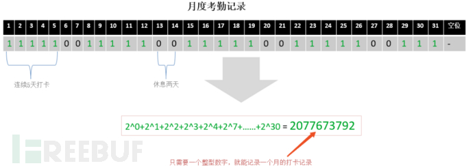
・Using bitwise operations to implement application scenarios such as switch and multiple option superposition (resource permissions). An int type has 32 bits, theoretically capable of representing 32 switch states or business options; taking the monthly sign-in scenario of a user as an example: an int field is used to represent the sign-in status of a user for a month, 0 indicating no sign-in, and 1 indicating sign-in. To determine if a user has signed in on a specific day, it is only necessary to check if the corresponding bit is 1. To calculate the total number of sign-ins in a month, simply count the number of bits that are 1. This clever data storage structure will be introduced in more detail in the bitmap (BitMap) later.
・Implement business priority calculation using bitwise operations:
public abstract class PriorityManager {
    // Define business priority constants
    public static final int PRIORITY_LOW = 1;     // Binary: 001
    public static final int PRIORITY_NORMAL = 2;  // Binary: 010
    public static final int PRIORITY_HIGH = 4;    // Binary: 100

    // Define user permission constants
    public static final int PERMISSION_READ = 1;  // Binary: 001
    public static final int PERMISSION_WRITE = 2; // Binary: 010
    public static final int PERMISSION_DELETE = 4; // Binary: 100

    // Define the combination value of user permissions and business priorities
    public static final int PERMISSION_LOW_PRIORITY = PRIORITY_LOW | PERMISSION_READ;     // Binary: 001 | 001 = 001
    public static final int PERMISSION_NORMAL_PRIORITY = PRIORITY_NORMAL | PERMISSION_READ | PERMISSION_WRITE;  // Binary: 010 | 001 | 010 = 011
    public static final int PERMISSION_HIGH_PRIORITY = PRIORITY_HIGH | PERMISSION_READ | PERMISSION_WRITE | PERMISSION_DELETE;  // Binary: 100 | 001 | 010 | 100 = 111

    // Determine if the user's permission meets the business priority requirements
    public static boolean checkPermission(int permission, int priority) {
        return (permission & priority) == priority;
    }
}
• Other typical scenarios using bit operations: the design of queue length in HashMap, and the use of AtomicInteger field ctl in ThreadPoolExecutor to store the current thread pool status and thread count (the high 3 bits represent the current thread status, and the low 29 bits represent the number of threads).
4.2.2 BitMap
BitMap (BitMap) is a commonly used data structure with wide applications in indexing, data compression, etc. The basic idea is to use a bit to mark the corresponding Value of an element, and the Key is the element itself. Since it stores data in bits, it can greatly save storage space and is a rare data structure that can ensure both storage space and search speed (without trading space for time).
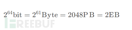
For example, suppose there is such a requirement: find out whether a number m exists among 2 billion random integers, and assume a 32-bit operating system, 4G memory, in Java, int occupies 4 bytes, 1 byte = 8 bits (1 byte = 8 bit).
• If each number is stored with int, that would be 2 billion ints, thus occupying space about (2000000000*4/1024/1024/1024)≈7.45G
• If stored bit by bit, 2 billion numbers would be 2 billion bits, occupying space about (2000000000/8/1024/1024/1024)≈0.233G
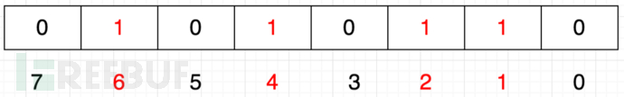
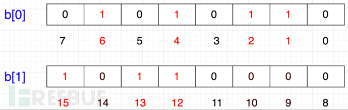
Storage space can be compressed and saved by 31 times! So how does it achieve digital marking through binary bits? The principle is to use each binary bit (index) to represent a real number, 0 to represent the absence, and 1 to represent the existence. In this way, we can easily represent the numbers {1,2,4,6}:
The minimum unit of memory allocation in a computer is a byte, which is 8 bits. So how to represent {12,13,15}? You can apply for another byte b [1]:
A two-dimensional array is used to implement bit addition. Since 1 int occupies 32 bits, we only need to apply for an int array with a length of int index [1+N/32] to store, where N represents the maximum value of the numbers to be stored:
index [0]: It can represent 0~31
index [1]: It can represent 32~63
index [2]: It can represent 64~95
By analogy... In this way, given any integer M, M/32 gets the index, and M%32 knows which position it is at this index.
BitMap data structure is usually used in the following scenarios:
1. Compression of a large number of boolean values: Bitmap can effectively compress a large number of boolean values, thereby reducing memory usage;
2. Fast judgment of the existence of an element: Bitmap can quickly determine whether an element exists, just by looking up the corresponding bit;
3. De-duplication: Bitmap can be used for de-duplication operations, where elements are used as indexes, and the corresponding bits are set to 1. Duplicate elements will only correspond to the same bit, thus achieving de-duplication;
4. Sorting: Bitmap can be used for sorting, where elements are used as indexes, and the corresponding bits are set to 1. Then, by traversing the bit array in the order of the index, an ordered sequence of elements can be obtained;
5. In the design of search pruning in search engines such as ElasticSearch and Solr, it is necessary to save the historical information of the searched data, and Bitmap can be used to reduce the space occupied by historical information data;
4.2.3 Bloom Filter
Bitmap, this data storage structure, if the data volume is large enough, such as 64-bit data types, a simple calculation of the storage space shows that the massive hardware resources required are no longer realistic:
Therefore, another famous industrial implementation —— Bloom Filter (Bloom Filter)It has appeared. If BitMap maps each possible integer value through direct addressing, which is equivalent to using a hash function, then the Bloom filter introduces k (k>1) independent hash functions to ensure that the element de-duplication process is completed under the given space and error rate. The figure below is a Bloom filter with k = 3:
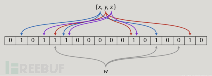
The internal mechanism of the Bloom filter relies on hash algorithms. When checking whether a piece of data has been seen before, there is a certain probability of false positives (False Positive), but there will never be false negatives (False Negative). That is to say, when the Bloom filter considers a piece of data as having appeared, it is very likely that the data has appeared; however, if the Bloom filter considers a piece of data as not having appeared, then the data is definitely not present. The Bloom filter introduces a certain error rate to enable the heavy data to be judged within the acceptable memory cost.
In the figure above, x, y, z are mapped to three positions in the Bitmap by the hash function and set to 1, when w appears, it only indicates that w is in the set when all three flags are 1. In the shown situation, the Bloom filter will determine that w is not in the set.
Common implementation
・Implementation in the Guava utility package in Java;
・Starting from Redis 4.0, the Bloom filter feature is provided as a plugin;
Applicable scenarios
・Web crawler de-duplicates URLs to avoid crawling the same URL addresses, for example, Chrome browser uses a Bloom filter to identify malicious links;
・Spam email filtering: determine whether a certain email is a spam email from a list of tens of billions of spam emails;
・Solve database cache collision: when hackers attack the server, they will build a large number of keys that do not exist in the cache and send requests to the server. When the data volume is large enough, frequent database queries can lead to hanging;
・Google Bigtable, Apache HBase, Apache Cassandra, and PostgreSQL use Bloom filters to reduce disk searches for non-existent rows or columns;
・Check if the user has purchased repeatedly in the flash sale system;
4.3 Circular Queue
A circular queue is a data structure used to represent a fixed-size, head-to-tail connected structure, which is very suitable for caching data streams. It is present in various scenarios such as communication development (Socket, TCP/IP, RPC development), inter-process communication (IPC) in the kernel, video and audio playback, and so on. Various middleware used in daily development, such as Dubbo, Netty, Akka, Quartz, ZooKeeper, and Kafka, also incorporate the concept of circular queues. Below, two commonly used circular data structures are introduced: the hash ring and the time wheel.
4.3.1 Consistent Hash Ring
Let's take a look at the structure of a typical hash algorithm first:
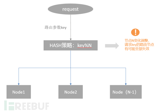
Taking the Hash strategy in the figure as an example, when the number of nodes N changes, almost all previous hash mappings are invalidated. If the cluster is a stateless service, there is nothing much to worry about. However, in scenarios such as distributed caching, it can lead to serious problems. For example, Key1 was originally routed to Node1, and the Value1 data in the cache was hit. However, after the change of N nodes, Key1 may be routed to Node2, which leads to the problem of cache data not being hit. Whether it is machine failure or cache expansion, it will lead to changes in the number of nodes.
How to solve the problem in the above scenario? It is the consistent hash algorithm to be introduced next.
Consistent hashing organizes the entire hash value space into a virtual circle. Assuming the value space of a hash function H is 0-2^32-1 (i.e., the hash value is a 32-bit unsigned integer), all input values are mapped to the range of 0-2^32-1 to form a circle. The entire hash space ring is as follows:
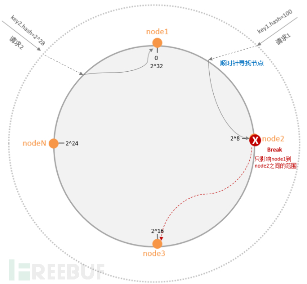
The process of routing data is as follows: The data key is calculated using the same Hash function to determine the hash value, and the position of this data on the ring is determined. Starting from this position, 'travel' clockwise along the ring, the first node encountered is the server where it should be located. If a server at a node fails, the scope of its impact is no longer all clusters, but is limited to the area between the failed node and its upstream nodes.
When a node fails, all the requests originally belonging to it will be re-hashed and mapped to the downstream nodes, which may cause the downstream nodes to be overloaded and possibly fail, thus easily forming a cascade. To solve this problem, virtual nodes are introduced.
Many virtual nodes are distributed on the circle according to the Node node, and each real node maps to multiple virtual nodes. In this way, when a node fails, the requests originally belonging to it are evenly distributed to other nodes, which reduces the risk of a cascade and also solves the problem of uneven request distribution caused by a small number of physical nodes.
Hash ring with virtual nodes:
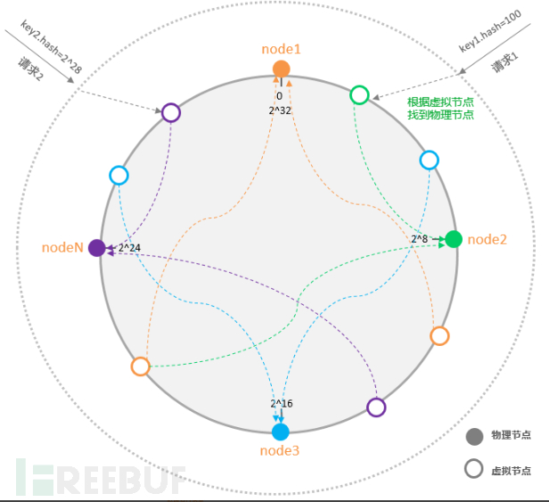
Consistent Hash algorithm is widely used in the load balancing field due to its characteristics of balanced and persistent mapping, such as nginx, dubbo, etc., which all have consistent hash implementations internally.
4.3.2 Time Wheel Slicing
The TimeWheel is a sophisticated algorithm for implementing delay functions (timers) and can realize an efficient delay queue. Taking the TimeWheel implementation scheme in Kafka as an example, it is a circular queue for storing scheduled tasks, and the underlying implementation uses an array. Each element in the array can store a list of scheduled tasks (TimerTaskList). The TimerTaskList is a circular doubly linked list, and each item in the list represents a scheduled task item (TimerTaskEntry), which encapsulates the actual scheduled task TimerTask.
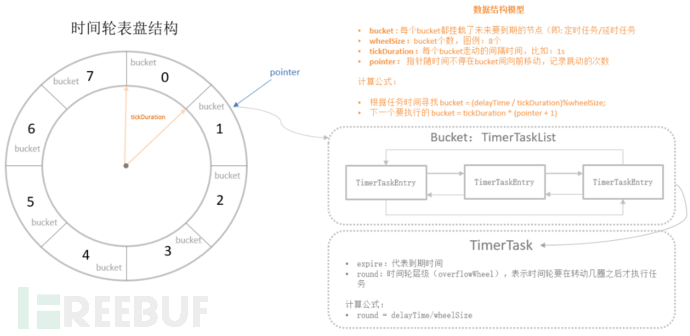
From the above figure, it can be found that the time wheel algorithm no longer uses a task queue as a data structure, and the polling thread is no longer responsible for traversing all tasks, but only traverses the time scales. The time wheel algorithm is like a pointer constantly rotating and traversing on a clock, and if it finds a task (task queue) at a certain moment, it will execute all tasks on the task queue.
Assuming the interval between adjacent bucket expiration times is bucket=1s, starting from 0s, the scheduled tasks that expire after 1s are hung under bucket=1, and the scheduled tasks that expire after 2s are hung under bucket=2. When checking that 1s has passed, all nodes under bucket=1 execute timeout actions, and when the time reaches 2s, all nodes under bucket=2 execute timeout actions. The time wheel uses a pointer on a dial to represent the number of times the pointer jumps, which can be represented by tickDuration * (pointer + 1) to indicate the next due task, and all tasks in the corresponding TimeWheel bucket need to be processed.
Advantages of the time wheel
1. The addition and removal of tasks are both O(1) complexity;
2. Only one thread is needed to advance the time wheel, which does not consume a large amount of resources;
3. Compared with other task scheduling modes, the load on CPU and resource waste are reduced.
Applicable scenarios
The time wheel is a scheduling model produced to solve the problem of efficient task scheduling. It can be effective in scenarios such as periodic timing tasks, delayed tasks, and notification tasks.
V. Summary
This article explains the names and concepts related to data storage, focusing on the development history of database technology. In order to enrich the readability and practicality of the article, it also extends some technical practical capabilities from the perspective of data structure design, expounds the application of related data structures such as linked lists, bitwise operations, and circular queues in the field of software development, and hopes that this article will bring you benefits.
Note: Some of the images in this article are from the Internet
hacker hire iiit hyderabad(IIIT Hyderabad)
Database入门:Master the five basic operations of MySQL database and easily navigate the data world!
Git leak && AWS AKSK && AWS Lambda cli && Function Information Leakage && JWT secret leak
III. Real-time operating system based on Linux

评论已关闭